Introduction: Noise is Everywhere
Imagine yourself sitting in a noisy laboratory, writing code. People around you are chatting, and countless devices are humming. While sometimes you wish those chatty people would just “shut up,” there’s a more elegant solution: filter out all the information you don’t care about.
Filtering is one of the most common operations in signal processing. It can be extremely simple or incredibly complex, depending on what you want to filter. Today, let’s discuss the simplest type: the First-Order Infinite Impulse Response (IIR) Low-Pass Filter, sometimes also called the Exponential Moving Average Filter.
A Typical Filtering Problem
Let’s use a concrete example to illustrate the necessity of filtering. Suppose we have a desired signal with a frequency of 50Hz, but the received signal is mixed with high-frequency noise at 5000Hz (in real applications, the noise spectrum is much richer; this is just for demonstration):
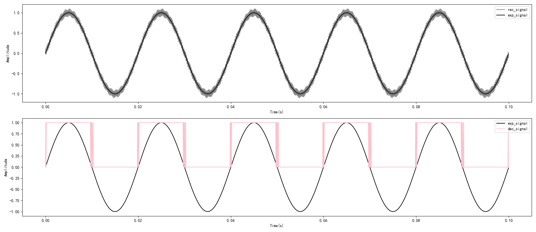
The above shows a zero-crossing detection scenario. If we directly use the noisy received signal (rec_signal) for detection, the result (dec_signal, pink line) is completely unusable—noise causes numerous false triggers.
A harsh reality is: noise is almost inevitable in embedded applications, especially when dealing with analog signals. So how do we get rid of this noise?
The answer might lie in the hardware engineer’s toolbox.
From RC Filter to Digital World
This is a classic RC low-pass filter circuit:
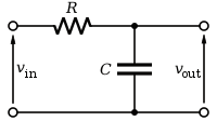
The working principle of this circuit is clever: the capacitor presents low impedance to high-frequency signals (acting like a short circuit), while presenting high impedance to low-frequency signals, allowing the signal to primarily flow to the load. The values of the resistor and capacitor determine the cutoff frequency—the dividing point.
Hardware engineers often use this circuit to filter out high-frequency noise. The good news is that we can use mathematics to “translate” this analog circuit into digital code!
Mathematical Derivation
The differential equation of this circuit is not difficult to write:
$$ \frac{dV_{out(t)}}{dt} = \frac{1}{RC}\left(V_{in(t)}-V_{out(t)}\right) \tag{1} $$
Applying Laplace Transform:
$$ sV_{out(s)} = \frac{1}{RC}\left(V_{in(s)}-V_{out(s)}\right) \tag{2} $$
We get the Transfer Function:
$$ \frac{V_{out(s)}}{V_{in(s)}} = \frac{1}{RCs+1} = \frac{1}{\tau s+1} \tag{3} $$
Where $\tau=RC$ is the time constant of the system. From the transfer function, we can see that the RC filter is a typical first-order linear system.
However, the above formula describes a continuous system. To implement it in a digital system, we need to perform discretization.
Discretization: From Continuous to Digital
With the powerful tool of Z-Transform, we can map the s-domain to the z-domain:
$$ s=\frac{1-z^{-1}}{T_{s}} \tag{4} $$
Where $T_s$ is the sampling period.
Substituting equation (4) into equation (3):
$$ \frac{V_{out(z)}}{V_{in(z)}} = \frac{1}{\tau\frac{1-z^{-1}}{T_{s}}+1} = \frac{T_{s}}{\tau(1-z^{-1})+T_{s}} \tag{5} $$
Rearranging:
$$ V_{in(z)} = (1+\frac{\tau}{T_{s}})V_{out(z)}-\frac{\tau}{T_{s}}V_{out(z)}z^{-1} \tag{6} $$
Inverse transforming back to the time domain:
$$ V_{in(n)} = (1+\frac{\tau}{T_{s}})V_{out(n)}-\frac{\tau}{T_{s}}V_{out(n-1)} \tag{7} $$
Finally, we get the discretized expression of the RC filter:
$$ V_{out(n)} = \frac{T_{s}}{T_{s}+\tau}V_{in(n)}+(1-\frac{T_{s}}{T_{s}+\tau})V_{out(n-1)} \tag{8} $$
A More Friendly Form
Let $a = \frac{T_{s}}{T_{s}+\tau}$, and the formula simplifies to:
$$ V_{out(n)} = aV_{in(n)} + (1-a)V_{out(n-1)} \tag{9} $$
So elegant! This formula tells us: current output = a small portion of input + a large portion of previous output.
To make the formula more practical, let’s express coefficient a in terms of frequency.
The relationship between time constant $\tau$ and cutoff frequency $f_c$:
$$ \tau = \frac{1}{2\pi f_{c}} \tag{10} $$
The relationship between sampling period $T_s$ and sampling frequency:
$$ T_{s} = \frac{1}{f_{s}} \tag{11} $$
So coefficient a can be written as:
$$ a = \frac{2\pi f_{c}}{2\pi f_{c}+f_{s}} \tag{12} $$
Code Implementation
Here’s the Python implementation:
1 | def lpf(x, fs, fc): |
Let’s see how it performs:
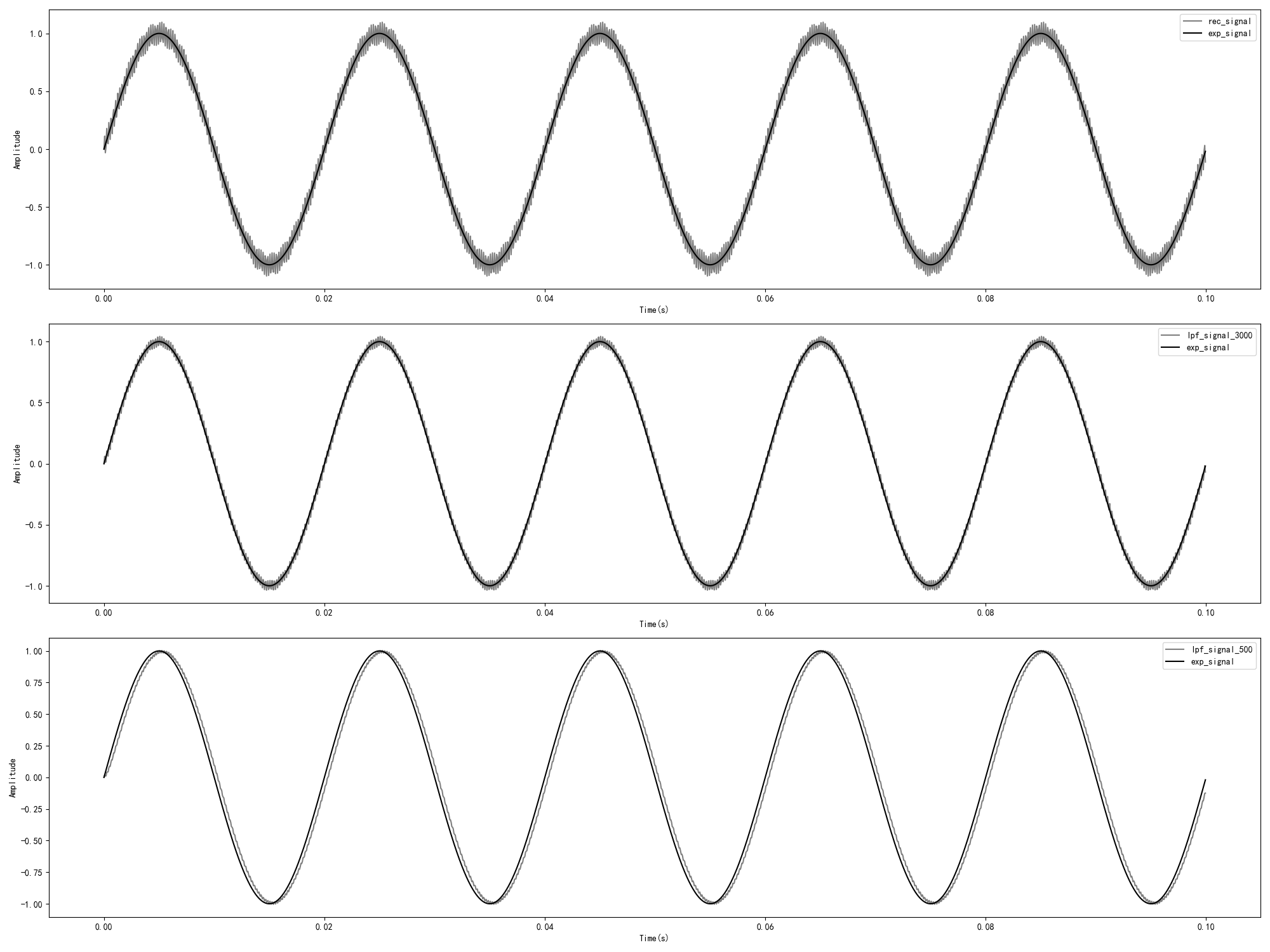
The above shows three scenarios:
- Original received signal (gray): mixed with 5000Hz noise
- fc=3000Hz filtering (middle): noise is reduced but still noticeable
- fc=500Hz filtering (bottom): noise almost disappears, signal is smooth
The lower the cutoff frequency, the more obvious the filtering effect, but it also brings more phase delay—this is a trade-off in engineering.
The Pitfall of Fixed-Point Implementation
So far, everything looks great. But there’s a problem: the code above uses floating-point operations.
In the embedded world, especially on low-end MCUs without an FPU (Floating Point Unit), floating-point operations are very expensive. We need to implement it using fixed-point arithmetic.
Fixed-Point Implementation
A naive approach is: scale all values by a certain factor, round to integers, use integer operations, and finally scale back.
1 | def lpf_fixp(x, q, fs, fc): |
Seems fine? Let’s look at the actual result:
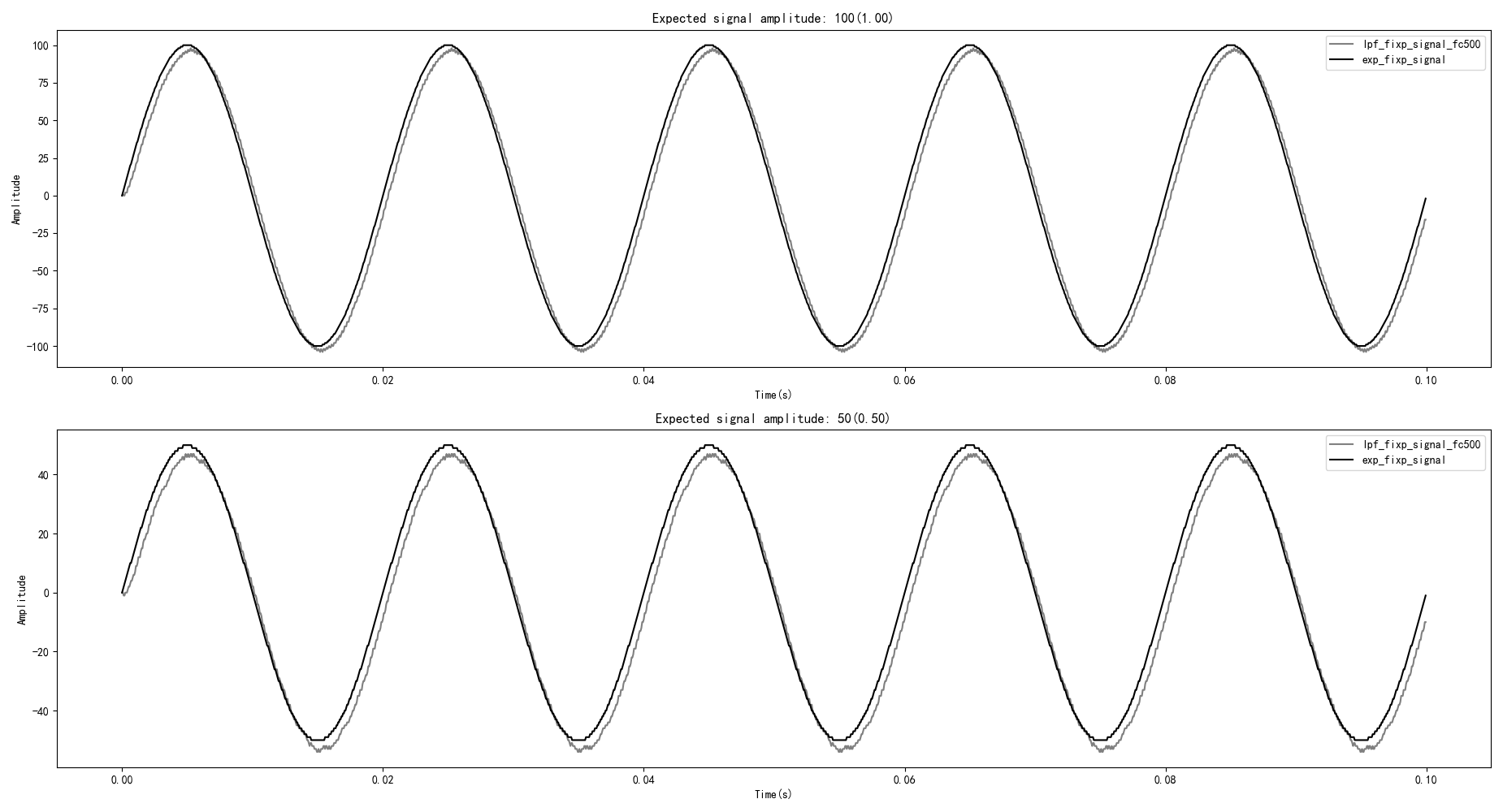
Oh no! The filtered signal shows a significant negative DC bias, and this problem becomes more severe as the signal amplitude decreases.
Root Cause of the Problem
To understand the problem, let’s first derive the fixed-point formulation from the basic filter equation.
Starting from the continuous form and applying fixed-point scaling:
$$ V_{out(n)} = \frac{(a_{scaled} \cdot V_{in(n)} + (IQN_1 - a_{scaled}) \cdot V_{out(n-1)})}{IQN_1} \tag{13} $$
Where:
- $IQN_1 = 1 << q$ (the scaling factor, where q is the number of fractional bits)
- $a_{scaled} = a \cdot IQN_1$ (the scaled filter coefficient)
This can be simplified to a more computationally efficient recursive form:
$$ V_{out(n)} = V_{out(n-1)} + \frac{a_{scaled} \cdot (V_{in(n)} - V_{out(n-1)})}{IQN_1} \tag{14} $$
Now, analyzing the naive fixed-point implementation formula carefully:
$$ V_{out(n)} = V_{out(n-1)} + ((a_{scaled}*(V_{in(n)} - V_{out(n-1)}))>>q) \tag{15} $$
The problem lies in the right shift operation! In fixed-point arithmetic, right shift is equivalent to division and loses precision.
When $|a_{scaled}*(V_{in(n)} - V_{out(n-1)})|$ is less than the shift amount, the result becomes 0. This means new inputs cannot correctly affect the output, leading to cumulative error.
Optimization Solution
The solution is: don’t shift too many bits at once. We do it in two steps:
- First shift right by n bits, ensuring no precision loss
- Accumulate to an intermediate variable
- Finally shift right by the remaining (q-n) bits
The key is choosing an appropriate n value. To ensure correct filter behavior, we must satisfy this critical constraint:
$$ (a_{scaled} \cdot 1) >> n \geq 1 \tag{16} $$
This constraint guarantees that when the smallest possible input (magnitude of 1) is scaled and shifted right by n bits, the result is still at least 1. This ensures that new samples—whether positive or negative—can correctly influence the filter output.
From this constraint, we can derive the upper bound for n:
$$ n \leq \log_2 a_{scaled} \tag{17} $$
The formula is modified to use a two-stage accumulation:
$$ V_{temp(n)} = V_{temp(n-1)} + ((a_{scaled}*(V_{in(n)} - V_{out(n-1)}))>>n) \tag{18} $$
$$ V_{out(n)} = V_{temp(n)}>>(q - n) \tag{19} $$
Optimized Code
1 | def lpf_fixp_Op(x, q, fs, fc): |
Comparison of results:
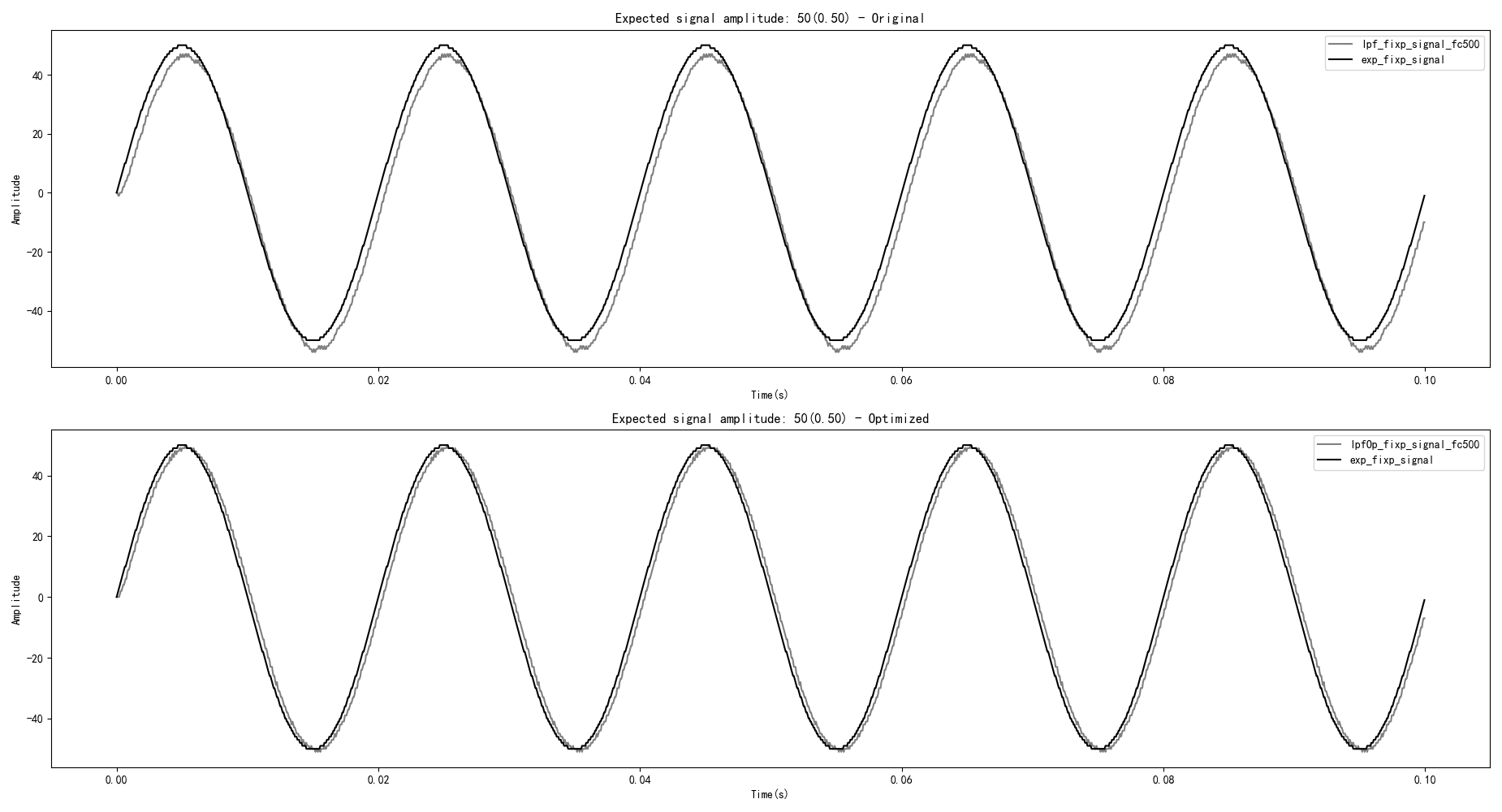
Perfect! The negative DC bias is gone, and the fixed-point filter works correctly.
Frequency Domain Analysis: Deeper Understanding
The previous analysis was based on the time domain (observing signal changes over time). In filter design and control systems, frequency domain analysis is more common—observing the attenuation of different frequency components.
Let’s use FFT to examine the signal spectrum:
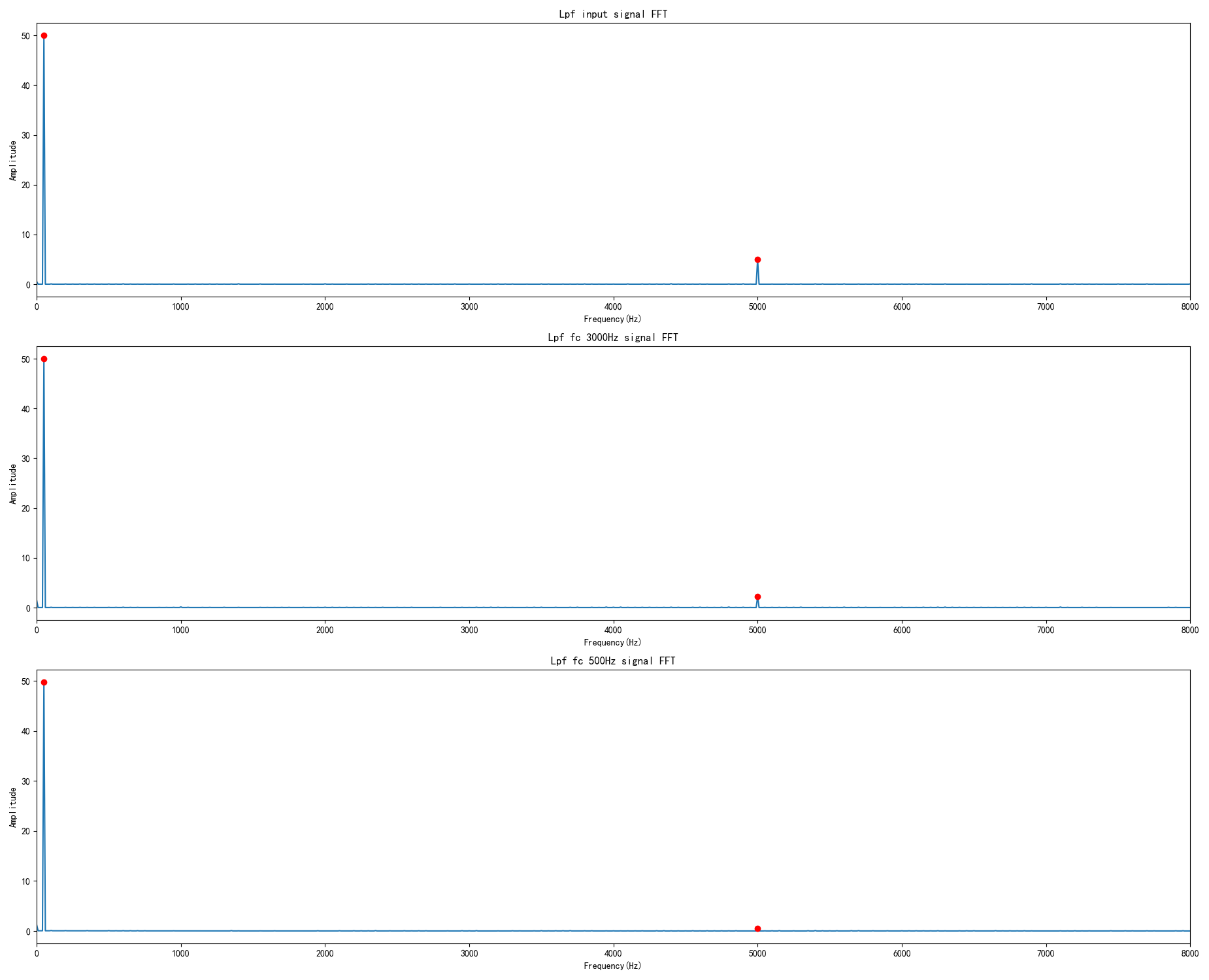
Figure: FFT spectrum analysis of signals before and after filtering. From the frequency domain perspective:
- Input signal contains strong 50Hz component (desired signal) and 5000Hz component (noise)
- After fc=3000Hz filtering: 5000Hz noise amplitude reduced from 1.0 to 0.514 (51.4% remaining)
- After fc=500Hz filtering: 5000Hz noise amplitude reduced from 1.0 to 0.100 (10% remaining)
- 50Hz signal remains essentially unchanged in both cases
Bode Plot: The “Fingerprint” of a Filter
The Bode plot is a standard tool for describing a filter’s frequency response. Let’s plot it:
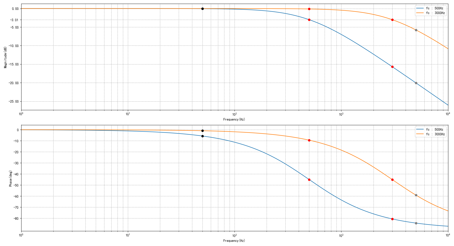
Figure: Bode plot comparison of first-order low-pass filters with cutoff frequencies at 500Hz and 3000Hz. The magnitude plot (top) shows attenuation in decibels, while the phase plot (bottom) shows phase shift in degrees. Key points: at cutoff frequency, gain = -3.01dB and phase = -45°.
Qualitative Analysis
From the Bode plot, we can draw four key conclusions:
Same cutoff frequency, different input frequencies: When comparing 50Hz vs 5000Hz signals filtered by the same cutoff frequency (e.g., fc=500Hz), the higher frequency signal (5000Hz) experiences much greater magnitude attenuation.
Same cutoff frequency, different input frequencies: For the same cutoff frequency, higher input frequencies result in more phase lag. The 5000Hz signal has significantly more phase shift than the 50Hz signal.
Different cutoff frequencies, same input frequency: When comparing different cutoff frequencies (fc=500Hz vs fc=3000Hz) filtering the same 50Hz signal, the lower cutoff frequency causes slightly more magnitude attenuation.
Different cutoff frequencies, same input frequency: For the same input frequency, lower cutoff frequencies produce more phase lag. The fc=500Hz filter introduces more phase shift than fc=3000Hz for all frequencies.
These four observations reveal the fundamental trade-off in filter design: lower cutoff frequencies provide better noise rejection but introduce more phase lag.
Several important conclusions can be drawn from the Bode plot:
| Characteristic | Description |
|---|---|
| Magnitude Response | For a fixed cutoff frequency, higher input frequencies experience greater attenuation. For a fixed input frequency, lower cutoff frequencies cause greater attenuation. |
| Phase Response | For a fixed cutoff frequency, higher input frequencies experience more phase lag. For a fixed input frequency, lower cutoff frequencies cause more phase lag. |
| At Cutoff Frequency | Gain is -3.01dB (output amplitude = 0.707 × input), phase shift is exactly -45° |
| Signal-to-Noise Ratio | With fc=500Hz: 50Hz signal has 0.5% attenuation, 5000Hz noise has 90% attenuation. With fc=3000Hz: 50Hz signal has 0.02% attenuation, 5000Hz noise has 48.6% attenuation. |
Quantitative Analysis
To better understand the filter’s behavior, here’s the complete frequency response data:
| Test Frequency | fc=500Hz Magnitude | fc=500Hz V_ratio | fc=500Hz Phase | fc=3000Hz Magnitude | fc=3000Hz V_ratio | fc=3000Hz Phase |
|---|---|---|---|---|---|---|
| 50Hz (signal) | -0.04 dB | 0.995 | -5.71° | -0.01 dB | 0.998 | -0.96° |
| 500Hz (cutoff) | -3.01 dB | 0.707 | -45.00° | -0.28 dB | 0.968 | -9.46° |
| 3000Hz (cutoff) | -15.23 dB | 0.173 | -80.54° | -3.01 dB | 0.707 | -45.00° |
| 5000Hz (noise) | -20.00 dB | 0.100 | -84.29° | -5.78 dB | 0.514 | -59.04° |
Key observations:
- 50Hz signal: Virtually unaffected by either filter (less than 1% attenuation)
- 5000Hz noise: fc=500Hz filter removes 90% of noise; fc=3000Hz filter removes 48.6%
- Trade-off: Lower cutoff frequency = better noise rejection but more phase lag
Let’s use specific data to illustrate:
| Frequency | fc=500Hz | fc=3000Hz |
|---|---|---|
| 50Hz desired signal | 0.5% attenuation, 5.7° phase shift | 0.02% attenuation, 0.96° phase shift |
| 5000Hz noise | 90% attenuation | 48.6% attenuation |
Designing a filter is all about trade-offs:
- Noise sensitive → choose lower cutoff frequency, sacrifice phase
- Phase sensitive → choose higher cutoff frequency, tolerate more noise
Practical Recommendations
Based on the previous analysis, here are some engineering practical tips:
- Q value selection: Determines the calculation accuracy of the actual filter cutoff frequency, also affects overflow risk
- Nyquist theorem: Cannot filter noise above half the sampling frequency
- Shift bits: Must satisfy $n \leq \log_2 a_{scaled}$, otherwise quantization error will occur
- Phase consideration: The lower the cutoff frequency, the more serious the phase shift; use caution in phase-sensitive applications
More Advanced Filters
Sometimes, like a greedy teenager, we want it all—both no attenuation and phase shift in the desired signal frequency band, and sufficient gain reduction in the noise frequency band.
This requires more complex filters:
- Butterworth Filter: Flattest passband
- Chebyshev Filter: Steepest transition band
- Elliptic Filter: Best overall performance
- Kalman Filter: Optimal estimation based on state space
Of course, those are stories for another time…
Conclusion
The first-order digital low-pass filter is one of the most commonly used tools in embedded development:
- Simple principle: Just two multiplications and one addition
- Easy implementation: Both floating-point and fixed-point code are concise
- Significant effect: Effectively suppresses high-frequency noise
- Need attention: Precision issues in fixed-point implementation and phase delay
Remember that core formula:
$$ y[n] = a \cdot x[n] + (1-a) \cdot y[n-1] $$
Simple, elegant, practical.
References: